Deep Autoregressive Models

Forecasting with TensorFlow 2.0

Business-related time series are often non-continuous, or discrete, time-based processes. Operationally, it might be useful for businesses to know, or to be able to quantify when a time series will be at a peak or trough in the future. The goal is to capture the trend and periodic patterns and to forecast the signal for >1 samples into the future. The example notebook is available in the TensorFlow Formulation section of this article.

Trend, Periodicity, and Noise

n most business-related applications, the time series have non-constant mean and variance over time, or they can be said to be non-stationary. This is contrasted to stationary signals and systems used in the analysis of electrical circuits, audio engineering, and communication systems. The direction in which the mean value changes indicates the trend of the time series. The variation of the noise could be a function of some random process. The noise can potentially increase or decrease as a function of time.

There is a granularity time limit to the which periodic, or recurring, patterns can be captured. In digital signal processing, the Nyquist rate is the minimum sampling period required to capture a pattern that reoccurs with period N. Essentially, the sampling rate needs to be less than half of one cycle of the recurring pattern. For example, let us say there is a feature in the data that measures the number of sales every 6 hours. The most granular pattern that can be captured will be one that reoccurs every 12 hours.

Autoregressive Model Formulation

Autoregressive models and open loop feedback systems, a type of control system, have some similarities. Both of these systems depend on the previous output of the model. We would like both of these systems to be stable, i.e., not explode into an exponential output. These systems are different in that autoregressive forecasts can depend on multiple lagged input features. The form of the autoregressive model is shown in equation (0).

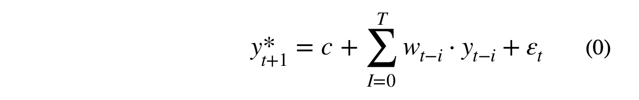
Where T is number of lagged features, w represents the autoregressive weights, y(t-i) represents the lagged time series, and y*(t+1) is the predicted value at t+1.

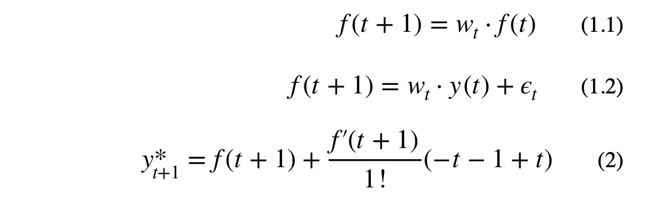
The goal is to create a linearized form of the autoregressive model using the 1st order Taylor Series approximation. The autoregressive formula is recursive, meaning the next value depends on a cascade of the previous values. The value at y(t+1) is estimated with Taylor Series expansion of f(t+1) around time step t. Equation (2) shows the estimated value for y(t+1) using the 1st order Taylor Series approximation. Note, that the -1 constant, on the right hand side of equation (2), will be absorbed by the weights.

Where f(t) is a recursive dense layer which represents y(t) with some error term, y* is the predicted output, w_t are the weights, and T is number of lagged features. Equation (3) shows the Taylor Series expansion for the simple case where y(t+1) depends on the previous value of f(t+1).The reason why I used f(t), in equation (2), instead of using y(t) directly is because y(t) represents the actual lagged data points, not a time dependent function.

Notice that, in equation (3.1), we took the partial derivative of f(t+1) with respect to f(t) and with respect to w(t). This partial derivative would result in f(t), which is another function that can be expanded with the 1st order Taylor Series expansion. Interestingly, this would result in the same AR model form, with the only difference being an infinite number of lagged features.

(3.2) can be reformulated as linear model by replacing the approximation function, f(t), with previous time series values for each lagged time step, i.e., the value of f(t-1) is replaced with y(t-1).

The final form used to train the autoregressive model is shown in equation (4). The intercept is constrained to be the sum of the autoregressive weights. This allows the model to be unbiased towards a central tendency and to be adaptive over time.

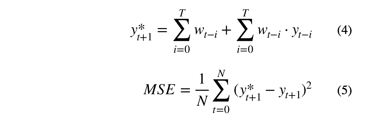
Where N is the number of data points, T is total number of lagged features, w represents the autoregressive weights, y(t-i) represents the lagged time series, and y*(t+1) is the predicted value at t+1. The objective function, MSE, shown in equation (5), is differentiable with respect to the parameters and can be optimized with TensorFlow.

Multi-variate time series can be forecasted by applying this same logic. The previous values for all time series are used as covariates to simultaneously predict the next value for all time series. In this case, the intercept is the sum of the output node’s autoregressive weights. The multivariate formulation allows for multiple autoregressive layers to be stacked to create a deep autoregressive model.

Daily Minimum Temperature and Rainfall in Melbourne, Australia

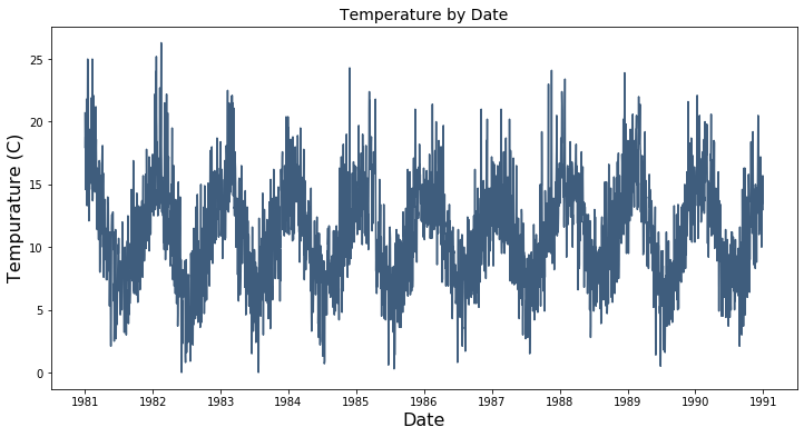
Daily Minimum Temperature and Rainfall in Melbourne, Australia dataset was used to build an autoregressive forecasting model. This dataset includes the Temperature and Rainfall across 3625 days, starting in 1981. There were a few missing values, but these values were interpolated for each series. These series were simultaneously forecasted using a deep autoregressive model.

Temperature

The plot below shows Temperature in Melbourne across the time frame. There appears to be a clear periodic component to Temperature over time.

<

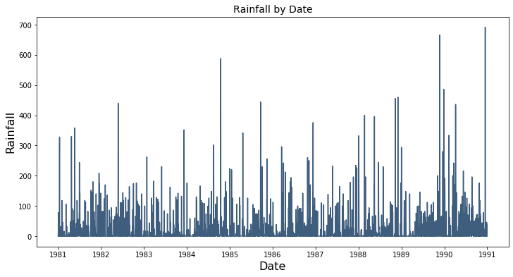
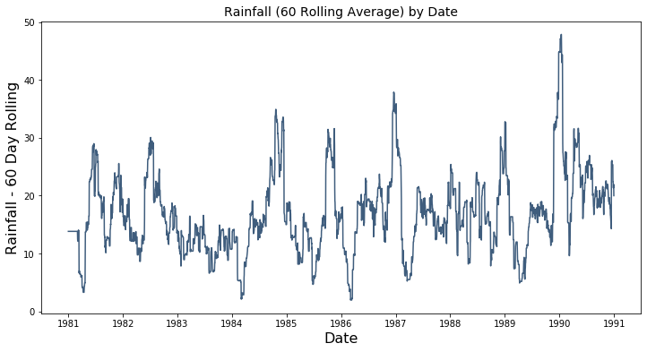
Rainfall

The plot below shows the Rainfall series, in Melbourne across the time frame. Rainfall is clipped at zero centimeters of rain per day which makes it difficult to model using an autoregressive model. In order to use Rainfall, a 60 rolling average for rainfall, shown in the second plot below, was created.

Dataset Construction

1. The two series, i.e., Temperature and Rain, were first standardized prior to training.
2. The dataset was constructed by creating 365 lagged features for each observation in the time series. For example, observation 365+1 will have the previous 365*2 features.
3. The first 365 observations were excluded from the training dataset to avoid missing values.
4. The last 1,130 observations, or 3 year, for both time series was used as the hold-out set to test the efficacy of the forecasts.

TensorFlow Formulation

The code block below shows the TensorFlow code for the autoregressive model formulated above. The example notebook can be found here.

The model has and input of size (N,M), where N is the number of data points and M corresponds to the 730 lagged features for both Rain and Temperature. A hidden layer of size 30 was used with autoregressive activation. The model was trained with stochastic gradient descent, mean squared error loss, an Adam optimizer, early stopping, and a small learning rate. While early stopping was utilized, it might not be necessary since the autoregressive model produces should be inherently regularized.

Snowballed Autoregressive Time Series

A forecast can be created by snowballing previous predictions into the autoregressive model. The variance of snowballed time series might have the tendency to increase across time, or become unstable, even if the actual time series is stable. A poorly fit model might become unstable and explode in variance across time. Instability can occur if the forecasted snowballed time series is consistently biased above or below the actual trend. The constrained intercept, in the model formulation, should produce more stability and adaptability over time.

In order to evaluate forecast stability, the model was trained 100 times on different, random train-validation splits, and 100 models were created. A snowballed time series was generated for each model on the hold-out set. The expected value and the standard deviation were used to create the forecast and confidence intervals, respectively.

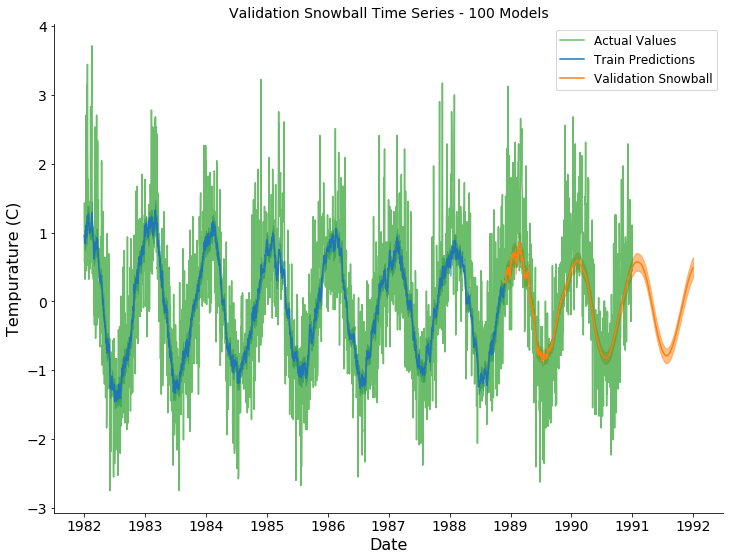
Temperature Forecast Result

Rainfall (60 Rolling Average) Forecast Result

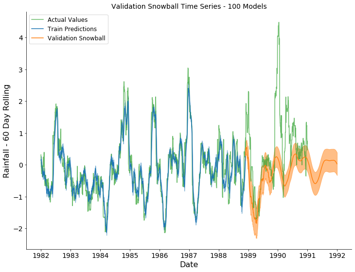
In the plots above, the actual observations, training predictions, and snowballed forecasts are shown by the green, blue, and orange series, respectively. The predicted and forecasted values for Temperature appear to capture the global periodic pattern. However, the variation across time was not captured by the variation across the 100 forecasts. The predicted values for Rainfall (60 rolling average) appear to be overfit on the training dataset. The overfitting might be due to the use of a rolling average feature. The trend , for this series, was accurately captured for ~1 year of forecasted values before collapsing into a periodic pattern. The trend was not accurately captured after ~1 year.

Conclusion

The 1st order approximation for the autoregressive function was used to formulate the objective function and the model definition. It was found that the intercept for the autoregressive activation layer was constrained to be the sum of the input’s weights. A deep autoregressive model was created using TensorFlow 2.0 by stacking autoregressive layers. The model was used to simultaneously forecast Temperature and Rainfall in Melbourne AU. The autoregressive formulation did not work with clipped time series, and a rolling average transformation was need to forecast Rainfall. The forecasts were created by snowballing the previous predictions back into the model. Small global trends and periodic patterns appeared to be captured by the model.

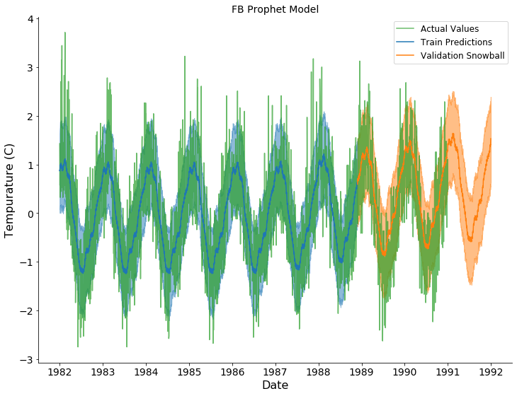
FB Prophet Forecast Comparison

How does the model stack up against FB Prophet? Prophet is a complete time series forecasting suite with many tunable parameters. For the comparison, I used the out of the box model from the quick start tutorial.

Prophet seems to use a periodogram model. It basically picks out the top periodic frequencies, f, and wraps them in sin and cosine functions to create the feature set, i.e., sin(f) and cos(f). The package also seems to also use the output of a logistic regression model. The logistic regression model predicts whether the series will go up or down. The package seems to support adding additional variables to the forecast, but it doesn’t seem to support simultaneous multi-variate forecasting yet. The comparison was added to the example notebook.

Temperature Forecast Result

Rainfall (60 Rolling Average) Forecast Result

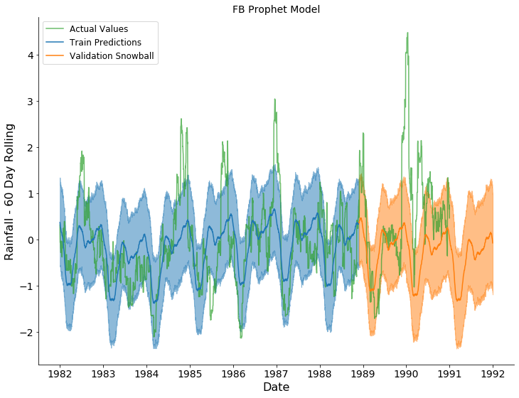
In the plots above, the actual observations, training predictions, and snowballed forecasts are shown by the green, blue, and orange series, respectively. The predicted and forecasted values for Temperature appear to capture the global periodic pattern. The variation across time was captured by the variation across the 100 forecasts. The trend for Temperature seems to trend upward which may not be the actual trend. The predicted values for Rainfall (60 rolling average) appear to capture a general, yearly periodic pattern. The pattern is consistent throughout the validation. The trend for Rainfall seems to trend downward which may not be the actual trend.