Autoregressive Models with TensorFlow
Autoregressive Models with TensorFlow
A time series can have different properties depending on the generating process and how the process is measured. There are many properties that describe a time series: 1) stationary 2) continuous 3) random 4) periodic. I’ll focus on non-random signals for this post, but I would recommend Applied Stochastic Processes, Chaos Modeling, and Probabilistic Properties of Numeration Systems By Vincent Granville, Ph.D. to anyone interested in random processes.
Most data scientist working with B2B or B2C time series are primarily working with non-continuous, or discrete, processes. Discrete means that the data are collected at fixed time intervals. If a time series has a recurring pattern, then the time series can be said to be periodic. The distiction between continuous and discrete is important because there is a granularity time limit to the which recurring patterns can be captured. In digitial signal processing, the Nyquist’s rate is the minimum sampling period required to capture a pattern with period N. Essentially, the sampling rate needs to be less than half of one cycle of the recurring pattern. For example, let us say there is a feature in the data that measures the number sales every 6 hours. The most granular pattern that can be captured will be one that reoccurs every 12 hours. In most business related applications, the time series have non-constant mean and variance over time, or are non-stationary. This is contrasted to the stationary signals and systems used in the analysis of electrical circuits, audio engineering, and communication systems. The problem with using signal processing on non-stationary processes is that it violates an assumption of the most fundamental signal processing algorithm, the Fourier transformation. “The Fourier transform assumes that the signal is stationary and that the signals in the sample continue into infinity. The Fourier transform performs poorly when this is not the case.” One potential solution is to use an autoregressive model.
Autoregressive Models
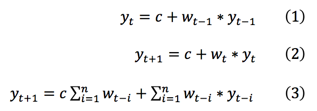
One thing that is really cool about autoregressive models is that they are similar to open loop feedback systems, a type of control system. The objective function for these models is buried under some heavy, almost nonsensical, mathematics, but I finally found a trick to build autoregressive models by searching Wikipedia. The trick can be summarized in the equations below by the following operations: insert (1) into (2) to create expression (3). The result of this transformation constrains the intercept to be some proportion of the autoregressive weights. This objective function can be optimized with TensorFlow. Please see the notebook for this post here.
The code block below shows how the weights and data were combined in TensorFlow for this model. The data was shaped into tuples of (N,M) input and output combinations, and the observations were split into training and testing datasets. The training dataset was shuffled. Stochastic mini batches, with 50% of the training observations, were used in each epoch. A gradient descent optimizer with a very small learning rate was used to prevent overfitting.
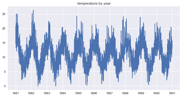
The autoregressive model was built using the daily minimum temperature in melbourne, Australia time series. This time series data did not need much preprocessing, i.e, only interpolating nan values. The clean dataset had ~3500 observations in total from which 80% was used for training.
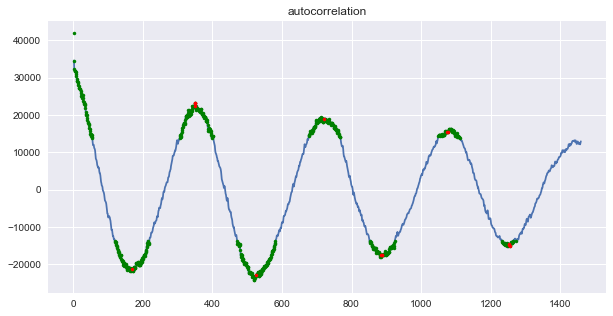
The auto correlation plot, shown below, was created with numpy’s correlate function by taking the last half of the correlations. The result was then detrended using scipy’s signal.detrend function. The plot below has peaks at the following lags: [170, 356, 528, 720, 897, 1079, 1257, 1455, 1622]. The strongest correlations were extracted by taking correlations at least two standard deviations from the mean correlation. In the plot below, the strongly correlated lags can be seen in green.
The input data was subsetted to exclude weakly correlated lags. This improved the quality of the input data by selecting only highly correlated lagged variable. These highly correlated lagged observations were extracted as a matrix for each target observation.
Snowballed Autoregressive Time Series
A forecast of the time series might be preferable when decisions need to be made some time in advance. A forecast can be created by ‘snowballing’ predictions into the autoregressive model. The variance of snowballed time series have the tendency to increase across time even if the actual time series has constant variance. A poorly fit model might become unstable and explode in variance across time. However, this increased variance is usually because the snowballed time series is above or below the actually trend of the time series. This seems to be an artifact of using an open loop system, as opposed to closed to systems which are used in electrical control systems. In order to test the randomness of the trend component direction, the model was trained with 1000 mini batches. The model results were saved for the last 900 epochs, and a snowballed time series was generated for each epoch.
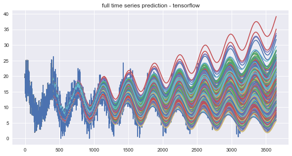
The snowballed time series by epoch are shown in the plot above. The trend’s randomness was tested by checking if the average error for each snowballed time series was above or below zero. There were roughly twice as many snowballed time series with positive trends than negative trends for the last 900, 600, and 300 epochs. The distributions of the average errors by epoch are shown in the histograms below.
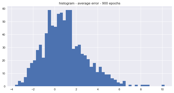
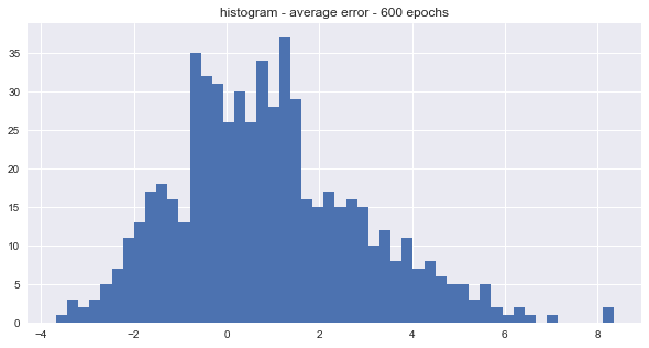
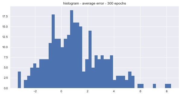
The average seems to be centered around 1 which means that most of the snowballed time series were over-predicting the actual values. The distribution seems to be slight right skewed too. However, it turns out that the snowball effect is not that large for medium range forecasts. One possible solution to the noise problem is to average N of the snowballed predictions together.
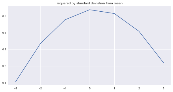
The last N lag components were used as predictors in the autoregressive model. Around 51% of the variation in the test data was explained when average ensembling the last 30 model from the last 30 epochs. The second plot, above, shows the r-squared by standard deviations from the mean of the snowballed time series. We can see that the r-squared is slightly more for the positive standard deviations (+1, +2, +3) that negative ones (-1, -2, -3) which suggests that the model might be over-predicting.
Predictions with the Actual Observations
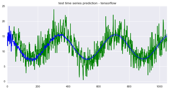
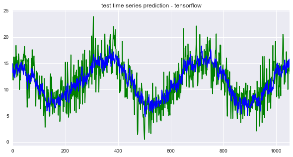
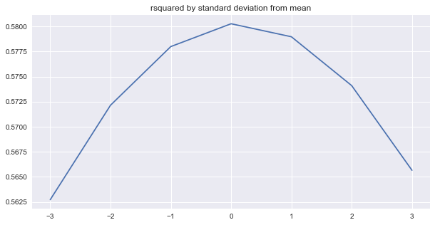
In contrast to forecasting, we can predict the next time step given the last N values for every observation in the test dataset. The predicted time series is shown below. Around 58%, 7% more than the snowballed prediction, of the variation in the test data was explained when average ensembling the last 30 epochs from the TensorFlow optimizer. Interestingly, the ‘r-squared by standard deviations from the mean’ plot suggests that the model might be over-predicting.
Conclusion
It is surprising how flexible TensorFlow layers can be. Additional model tuning and dataset could potential improve the results. For example, the number of hidden layers could be increased, additional predictors could be used, and regularization/intialization hyper parameters could be tuned. Rain fall per day is potentially a useful predictor for the target, temperature. The model performed reasonably well and adding these components added a significant amount project complexity.
I also built an autoregressive model with my custom optimizer, KernelML. I would argue that KernelML adds a little more modelling flexibility that can potentially lead to better model performance by making it easier to inject human intelligence into the model building process. My next blog post will show how using KernelML makes it easier to add more features and to make the model more complex, such as adding a feedback component (creating a closed-loop system).