Interesting Properties of the Covariance Matrix
The covariance matrix has many interesting properties, and it can be found in mixture models, component analysis, Kalman filters, and more. Developing an intuition for how the covariance matrix operates is useful in understanding its practical implications. This article will focus on a few important properties, associated proofs, and then some interesting practical applications, i.e., extracting transformed 2-D polygons from a Gaussian mixture's covariance matrix.
I have often found that research papers do not specify the matrices' shapes when writing formulas. I have included this and other essential information to help data scientists code their own algorithms.
Sub-Covariance Matrices
The covariance matrix can be decomposed into multiple unique (2x2) covariance matrices. The number of unique sub-covariance matrices is equal to the number of elements in the lower half of the matrix, excluding the main diagonal. A (DxD) covariance matrices will have D*(D+1)/2 -D unique sub-covariance matrices. For example, a three dimensional covariance matrix is shown in equation (0).
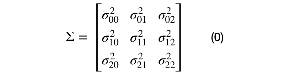
It can be seen that each element in the covariance matrix is represented by the covariance between each (i,j) dimension pair. Equation (1), shows the decomposition of a (DxD) into multiple (2x2) covariance matrices. For the (3x3) dimensional case, there will be 3*4/2–3, or 3, unique sub-covariance matrices.

Note that generating random sub-covariance matrices might not result in a valid covariance matrix. The covariance matrix must be positive semi-definite and the variance for each dimension the sub-covariance matrix must the same as the variance across the diagonal of the covariance matrix.
Positive Semi-Definite Property
One of the covariance matrix's properties is that it must be a positive semi-definite matrix. What positive definite means and why the covariance matrix is always positive semi-definite merits a separate article. In short, a matrix, M, is positive semi-definite if the operation shown in equation (2) results in a values which are greater than or equal to zero.

M is a real valued DxD matrix and z is an Dx1 vector. Note: the result of these operations result in a 1x1 matrix.
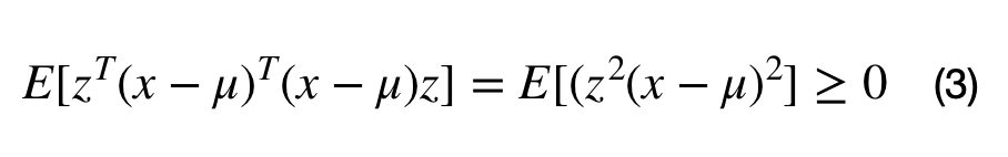
A covariance matrix, M, can be constructed from the data with the following operation, where the M = E[(x-mu).T*(x-mu)]. Inserting M into equation (2) lead to equation (3). It can be seen that any matrix that can be written in the form M.T*M is positive semi-definite. This full proof can be found here.
Note that the covariance matrix does not always describe the covariation between a dataset's dimensions. For example, the covariance matrix can be used to describe the shape of a multivariate normal cluster, for Gaussian mixture models.
Geometric Implications
Another way to think about the covariance matrix is geometrically. Essentially, the covariance matrix represents the direction and scale for how the data is spread. To understand this perspective, it will be necessary to understand eigenvalues and eigenvectors.
Equation (4) shows the definition of an eigenvector and its associated eigenvalue. The next statement is important in understanding eigenvectors and eigenvalues. Z is an eigenvector of M if the matrix multiplication M*z results in the same vector, z, scaled by some value, lambda. In other words, we can think of the matrix M as a transformation matrix that does not change the direction of z, or z is a basis vector of matrix M.

Lambda is the eigenvalue (1x1) scalar, z is the eigenvector (Dx1) matrix, and M is the (DxD) covariance matrix. A positive semi-definite (DxD) covariance matrix will have D eigenvalues and (DxD) eigenvectors. The first eigenvector is always in the direction of highest spread of data, all eigenvectors are orthogonal to each other, and all eigenvectors are normalized, i.e. they have values between 0 and 1. Equation (5) shows the vectorized relationship between the covariance matrix (sigma), eigenvectors, and eigenvalues.

S is the (DxD) diagonal scaling matrix, where the diagonal values correspond to the eigenvalue and which represent the variance of each eigenvector. R is the (DxD) rotation matrix that represents the direction of each eigenvalue.


The eigenvector and eigenvalue matrices are represented, in the equations above, for a unique (i,j) sub-covariance (2D) matrix. The sub-covariance matrix's eigenvectors, shown in equation (6), has one parameter, theta, that controls the amount of rotation between each (i,j) dimensional pair. The covariance matrix's eigenvalues are across the diagonal elements of equation (7) and represent the variance of each dimension. It has D parameters that control the scale of each eigenvector.
The Covariance Matrix Transformation
A (2x2) covariance matrix can transform a (2x1) vector by applying the associated scale and rotation matrix. The scale matrix must be applied before the rotation matrix as shown in equation (8).

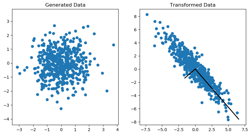
The vectorized covariance matrix transformation for a (Nx2) matrix, X, is shown in equation (9). The matrix, X, must centered at (0,0) in order for the vector to be rotated around the origin properly. If this matrix X is not centered, the data points will not be rotated around the origin.

An example of the covariance transformation on an (Nx2) matrix is shown in the Figure 1. More information on how to generate this plot can be found here.
Plotting Gaussian Mixture Contours
The contours of a Gaussian mixture can be visualized across multiple dimensions by transforming a (2x2) unit circle with the sub-covariance matrix. A contour at a particular standard deviation can be plotted by multiplying the scale matrix's by the squared value of the desired standard deviation. The clusters are then shifted to their associated centroid values.The code for generating the plot below can be found here.
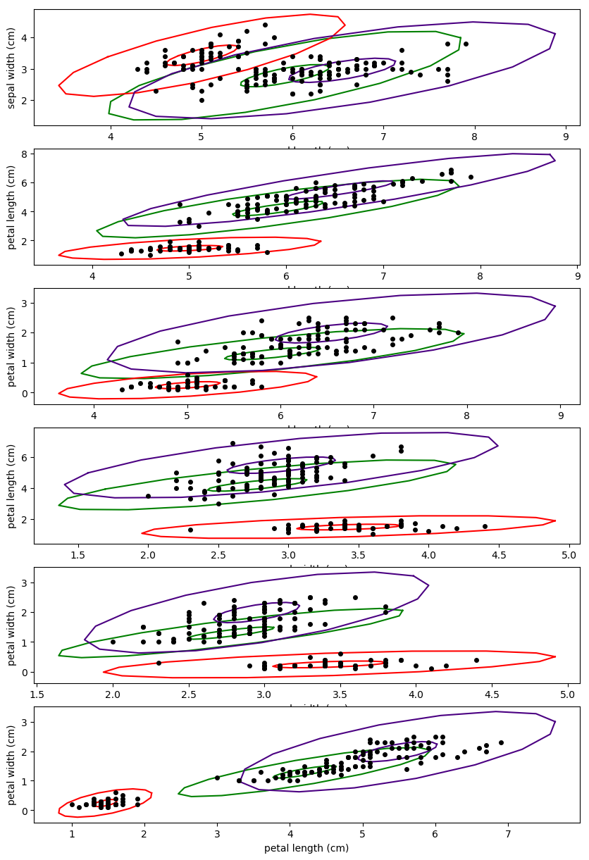
Figure 2. shows a 3-cluster Gaussian mixture model solution trained on the iris dataset. The contours represent the probability density of the mixture at a particular standard deviation away from the centroid. In Figure 2., the contours are plotted for 1 standard deviation and 2 standard deviations from each cluster's centroid.
Outlier Detection
Gaussian mixtures have a tendency to push clusters apart since having overlapping distributions would lower the optimization metric, maximum liklihood estimate or MLE. A data point can still have a high probability of belonging to a multivariate normal cluster while still being an outlier on one or more dimensions. A relatively low probability value represents the uncertainty of the data point belonging to a particular cluster.
A uniform mixture model can be used for outlier detection by finding data points that lie outside of the multivariate hypercube. These mixtures are robust to "intense" shearing that result in low variance across a particular eigenvector. It is also computationally easier to find whether a data point lies inside or outside a polygon than a smooth contour.
The uniform distribution clusters can be created in the same way that the contours were generated in the previous section. A unit square, centered at (0,0), was transformed by the sub-covariance matrix and then it was shift to a particular mean value.
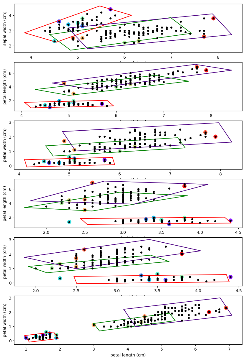
The rotated rectangles, shown in Figure 3., have lengths equal to 1.58 times the square root of each eigenvalue. Outliers were defined as data points that did not lie completely within a cluster's hypercube. The outliers are colored to help visualize the data point's representing outliers on at least one dimension. There are many different methods that can be used to find whether a data points lies within a convex polygon. Finding whether a data point lies within a polygon will be left as an exercise to the reader.
Another potential use case for a uniform distribution mixture model could be to use the algorithm as a kernel density classifier. The mean value of the target could be found for data points inside of the hypercube and could be used as the probability of that cluster to having the target. This algorithm would allow the cost-benefit analysis to be considered independently for each cluster.
Principal Component Analysis
Principal component analysis, or PCA, utilizes a dataset's covariance matrix to transform the dataset into a set of orthogonal features that captures the largest spread of data. The code snippet below hows the covariance matrix's eigenvectors and eigenvalues can be used to generate principal components.
The eigenvector matrix can be used to transform the standardized dataset into a set of principal components. The dimensionality of the dataset can be reduced by dropping the eigenvectors that capture the lowest spread of data or which have the lowest corresponding eigenvalues. The dataset's columns should be standardized prior to computing the covariance matrix to ensure that each column is weighted equally.
Final Notes
There are many more interesting use cases and properties not covered in this article: 1) the relationship between covariance and correlation 2) finding the nearest correlation matrix 3) the covariance matrix's applications in Kalman filters, and Mahalanobis distance 4) how to calculate the covariance matrix's eigenvectors and eigenvalues 5) how Gaussian mixture models are optimized.
Resources
Covariance and the Central Limit Theorem