KernelML is a particle optimizer that uses parameter constraints and sampling methods to minimize a customizable loss function. The package uses a Cythonized backend and parallelizes operations across multiple cores with the Numba. KernelML is now available on the Anaconda cloud and PyPi (pip). Please see the KernelML extention on the documentation page.

Density Factorization

The density factorization algorithm finds the peak values in an N-dimensional raster across 2-D manifolds. Note that the peak values are N dimensional vectors. The algorithm finds these peak values by optimizing the mean and variance of hyper-clusters. The estimated density can be of any aggregated statistic, i.e., counts, mean value, variance, max value, etc. Potential use cases are for peak detection, density estimation, and radial basis functions.

Data scientists and predictive modelers often use 1-D and 2-D aggregate statistics for exploratory analysis, data cleaning, and feature creation. Higher dimensional aggregations, i.e., 3 dimensional and above, are more difficult to visualize and to understand. High density regions, or concentrations of similar data points, are one example of these N-dimensional statistics. High density regions can be used for characterizing multiple groups in high dimensional space, outlier detection, assessing forecast plausibility. Other machine learning approaches such as clustering and kernel density estimation are similar, but these methods are different in a few important ways. It is worth noting why these methods, while useful, are not exactly designed for the purpose of finding these regions. The goal is to use KernelML to efficiently find the regions of highest density for an N-dimensional dataset.

My approach to developing this algorithm was to find a set of, common sense, constraints to construct the loss metric.

The density factorization algorithm, DF, algorithm uses N multivariate distributions to cluster the data. Normal or Uniform distributions can be used, but uniform distributions are less sensitive to outliers than normal distributions while normal distribution truncate correlations. This implementation uses uniform distributions. The most important aspect of these distributions is for the volume of each hyper-cluster to be "tied", or the same, with zero covariance. This helps with optimization efficiency and the goal of modeling densities not shapes. More clusters can always be added to approximate complex shapes. The video below shows the DF algorithm in action on a toy dataset.

Density Clustering with Gaussian Mixture Models

Clustering methods such as K-means and Gaussian mixture models, GMMs, use an iterative optimization algorithm that cycles between assigning data points to clusters and updating the cluster’s parameters. GMMs have a tendency to push clusters apart since having overlapping distributions would lower the optimization metric, maximum liklihood estimate or MLE. These clusters can grow in size and change shape which can be used to fit almost any arbitrary distribution. However, the scale and mean of the each cluster can be greatly influenced by skewed variables. Also, a data point can still be assigned to a cluster if it is dissimilar on a single dimension as long it is similar to the clsuter on the rest of the dimensions. The GMM optimization algorithm can be customized to keep the weight of each cluster equal to 1/N where N is the number of clusters. This will improve the representation of the estimated density and make the clusters easier to compare. The plots below show a comparison between the modified GMM, shown in the left plot, and the DF algorithm, shown in the right plot, on a multivariate normal mixture dataset with random uniform noise added to it. Notice how the GMM tends to push close clusters away and include outliers into the cluster solution.

It is possible to do a pull-request on scikit-learn’s current implementation of the Gaussian mixture model and modify the optimization procedure to keep equal weight on all clusters.

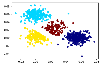
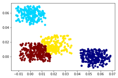
A cutoff threshold, for the normalized Mahalanobois distance, was found so that 80% of the data was clustered for both methods. Sklearn’s GaussianMixture class has an “_estimate_log_prob_resp” attribute that can be used to find the raw probabilities of an observation belonging to the closest cluster, i.e., the maximum exponential of the log probabilities. Notice how the Gaussian mixture solution tends to push close clusters away from each other. DF clusters are assigned data points only if the data points are within that cluster’s N-dimensional hyper-cube. Not all observations are within a hyper-cube cluster so a small variance scaling buffer can be added to the increase the size of each hyper-cube. If a data point lies within multiple hyper-cube clusters, the data point can be assigned to the closest DF cluster, where distance is calculated using a Chebyshev distance metric.

Kernel Density Estimation

Kernel Density Estimation, KDE, is a non-parametric method used to estimate the probability density of a “random variable” at a given data point. The estimator uses a smoothing parameter, h, to estimate the local density around a data point. The size of the smoothing parameter strongly effects the density estimate result. The DF creates an KDE for the cluster solution and then compared it to the data’s KDE. A larger smoothing parameter allows the hyper-cube DF cluster to cover more space in the KDE. Thus, the magnitude of the smoothing parameter is inversely proportional to the size of each density factorization cluster.

It is possible to estimate the points of highest density by performing a grid search of data points between the max-min of each dimension. However, this can be computationally expensive when the dimensionality of the data is high. The equation (1) shown the kernel density estimation equation.

The K function corresponds to a Gaussian kernel, h is the kernel's bandwidth, n is the number of data points, x is the dataset, and x_i is a grid point. The reason why using the KDE is impractical for estimating high density region can be seen in the following example: let's say we have a medium size dataset with 10,000 rows and 30 columns. If we search 15 data points between the max and min of each dimension, the density will need to be estimated for a total of 15³⁰ data points. The cost is multiplied by the, vectorized, operation(s) needed to compute the distances between each grid point and the rest of the dataset. After computing the highest points of density, a "peak clustering" algorithm would be needed to assign high density points to a region.

Density Factorization with KernelML

There are three main efficiency problems: 1) The DF clusters and the actual density manifolds, DM, need to be efficiently compared in an N-dimensional space 2) and the comparisons need to be efficient with respect to the number of data points.

Part 1) the DF cluster solution's and and the data's DM were compared by dividing the N-dimensional space into sets of 2-D slices. The density manifolds was computed for those slices. The loss metric can then be aggregated for each 2-D DM slice which reduces the computational complexity from N² to (N+1)*N/2 -N. Part 2) The 2-D DM can be estimated with a 2-D Gaussian filtered histogram. The filter makes each DM slice continuous and smooths out the loss function. Fast Fourier transforms can be used to compute the convolution between the Gaussian filter and the (histogram) DM. This further decreases the computational overhead. Part 3) There are many loss metrics that can compare the similarity between 2-D DM slices. Sum of squared errors is a good metric because it maximizes the error on large differences and minimizes the error on smaller differences. While the Kolmogorov Smirnov metric is commonly used to compare the cumulative distribution function (CDF) for 1-D distributions, it is non-trival to calculate the CDF of a multivariate distribution. The equation below (2), summarizes the loss metric used by the density factorization algorithm.

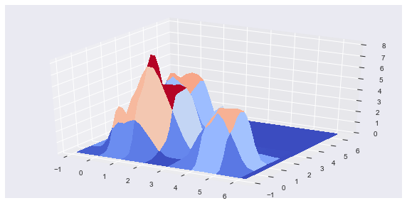
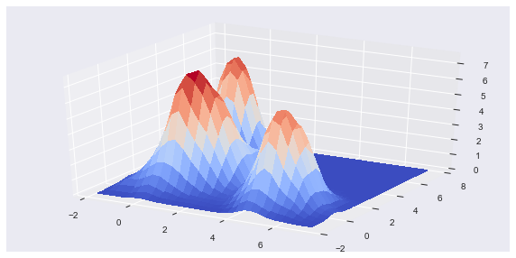
The loss metric takes the sum of squared errors between the 2-D DM slices for the cluster solution and the data. The DM slices are created and compared for unique dimensional pair combinations. Because the the DF clusters are uniform distributions, the DM can be easily filled in with a few data points and then L-1 normalized. The top plot, below, shows the Gaussian filtered HDRE cluster solution for the example shown in the video, in the first section. Notice how the jagged edges of the uniform distribution clusters are smoothed out. The bottom plot shows the DM for the original, multivariate Gaussian distributed, data.

Final Notes

Three criteria were used to evaluate the quality of each cluster solution: 1) the overall loss metric 2) the uniformity of cluster weights 3) the similarity of the observations to the cluster's centroid. The DF algorithm was added to KernelML as an extension. If you are interested in supporting KernelML's development and would like to add your own domain specific extension, I will be adding KernelML extensions in exchange for donations! I couldn't find many resources on this particular topic. I credit the term "high density regions" to the paper below. Please see this article on datasciencecentral.com for a different perspective on the deconvolution of statistical distributions with mixture models.

Fadallah, A. "High Density Regions for Uni- and Bivariate Densities." https://thesis.eur.nl/pub/9449/9449-Fadallah.pdf Rotterdam, 6 July 2011