DataScienceCentral.com - Complex Time Series Challenge
Rohan Kotwani
The original problem statement was given here
There was also a verbal solution given in the members only section. I'm not sure if its legal to share the whole thing, but here is an excerpt of the solution. " The time series has a weekly periodicity with two peaks: Monday and Thursday, corresponding respectively to the publication of the Monday and Thursday digests. The impact of the Monday and Thursday email blasts extent over the next day; this makes measuring the yield more difficult, unless you use additional data, e.g. from our newsletter vendor. However, the bulk of the impact is really on Monday and Thursday."
There are a variety of signal processing techniques that can be applied to time series data. For example, trend components can be extracted from a time series by transforming the signal into the frequency domain, filtering out non dominant frequencies, and then recombining the signal. This tends to work well for finding the overall trend, but it violates the assumption that the signal is a stationary process. In addition, this method is limited to the shapes that the sum of orthogonal sinusoids can make. This paper considers another approach where dominant frequencies are extracted, but where the signals are recombined in a linear model. In this linear model, the seasonality of the time series can be accounted by including a set of orthogonal sinusoidal waves, different frequencies, and different time components. However, finding the appropriate frequency and time component for each sinusoid requires a little more digging. This paper shows how to use Discrete Fourier transforms to automatically find these values.
Signal Processing Basics
- k ∈ [0,N-1] or k ∈ [-N/2, N/2-1] or k ∈ [-(N-1)/2, (N-1)/2]
- N = # of data points
- n = rank order of input data points
- k = rank order of output data points
Assumptions
"The Fourier transform assumes that the signal is stationary and that the signals in the sample continue into infinity. The Fourier transform performs poorly when this is not the case."
A stationary process has a constant mean and variance over time which is a property that most time series don't have. A stationary process can be extracted from the time series by creating a time differenced variable. However, the complex magnitudes from a time difference variable is not representatitve of the actual signal. A regression model can then be used to recontruct the magnitudes of this signal.
Model Definition
y = T(t) + S(t) + R(t)
- T(t)~Trend component
- S(t)~Seasonal component
- R(t)~Residual error
Objective function: minimize sum of squared errors
Closed form, least squared solution (Python code):
import numpy as np
A=x.T.dot(x) # x = intercept + predictor columns
b=x.T.dot(y) # y = target variable
z = np.linalg.solve(A,b)
This works perfectly for a dataset with a smaller number of non-collinear dimensions. However, the numpy algorithm can break with a dataset that has many collinear dimensions.
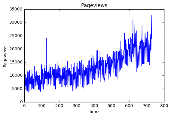
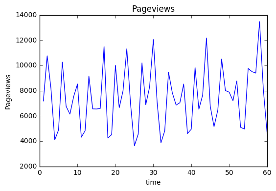
For the purposes of this post, we will only focus on the T(t) and S(t) components. 80% of the data or 584 observations were used to create the training set. The model was validated on the remaining 146 observations.
import pandas as pd
import numpy as np
import matplotlib.pyplot as plt
import datetime

full=pd.read_csv("DATA/DSC_Time_Series_Challenge.csv",dtype = {'Day ':str,'Sessions':int,'Pageviews':int})
time=[datetime.datetime.strptime(t[0],"%m/%d/%y") for t in full[['Day ']].values]
weekday=[datetime.datetime.strptime(t[0],"%m/%d/%y").isocalendar()[2] for t in full[['Day ']].values]

full['time']=time
full['index']=np.arange(1,len(full)+1)
full['weekday']=weekday
full=full.sort_values(by=['time'])

plt.plot(full['index'],full['Pageviews'],'-')
plt.xlabel('time')
plt.ylabel('Pageviews')
plt.title('Pageviews')
plt.show()
train=full[:580].copy()
valid=full[580:].copy()
train.head(n=5)
| Day | Sessions | Pageviews | time | index | weekday | |
|---|---|---|---|---|---|---|
| 0 | 9/25/13 | 4370 | 7177 | 2013-09-25 | 1 | 3 |
| 1 | 9/26/13 | 5568 | 10760 | 2013-09-26 | 2 | 4 |
| 2 | 9/27/13 | 4321 | 8171 | 2013-09-27 | 3 | 5 |
| 3 | 9/28/13 | 2378 | 4093 | 2013-09-28 | 4 | 6 |
| 4 | 9/29/13 | 2612 | 4881 | 2013-09-29 | 5 | 7 |
The weekday variable will be dummy coded and used later to compare results
weekday_dummies = pd.get_dummies(train.weekday, prefix='W').iloc[:, 1:]
train = pd.concat([train, weekday_dummies], axis=1)
weekday_dummies = pd.get_dummies(valid.weekday, prefix='W').iloc[:, 1:]
valid = pd.concat([valid, weekday_dummies], axis=1)
import Regression
import DSP
Finding the overall trend:
A polynomial term can be used to represent the trend component T(t) which can be created from the index variable. The complexity of the trend component can be tuned by using a training and validation set to find optimal complexity with the lowest sum of squared errors. A complexity of degree 2 had the lowest SSE value on the validation set so these terms will be included in the model.
heap = []
for i in range(1,15):
    z=Regression.sklearn_poly_regression(train[['index']],train[['Pageviews']],i)
    SSE = Regression.numpy_poly_regression_SSE(valid[['index']],valid[['Pageviews']],i,z)
    heap.append((SSE,i))
Regression.heapsort(heap)
    [(2501666772.2010365, 2),
     (2699152210.1621375, 9),
     (2699503808.6114817, 14),
     (2701796858.0785437, 10),
     (2701846050.0146337, 13),
     (2702552306.8232799, 12),
     (2706108691.5368271, 11),
     (2990342895.3898125, 8),
     (4491840385.0665913, 1),
     (4868690323.6375523, 4),
     (5963871838.3020554, 3),
     (11208662852.721825, 5),
     (317581251234.68689, 7),
     (477442016671.72321, 6)]
T_train = Regression.pandas_poly_feature(train[['index']],2)
T_valid = Regression.pandas_poly_feature(valid[['index']],2)
Removing the overall trend:
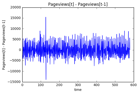
First, the overall trend needs to be removed from the signal in order to statisfy the stationary process assumption. This can be accomplished by creating a lag 1 differenced variable for Pageviews. This differenced variable will also make seasonal components easier to find.
time_diff_signal = DSP.time_diff_variable(train['Pageviews'],1)
plt.plot(train['index'][1:],time_diff_signal,'-')
plt.xlabel('time')
plt.ylabel('Pageviews[t] - Pageviews[t-1]')
plt.title('Pageviews[t] - Pageviews[t-1]')
plt.show()
The FFT transformation:
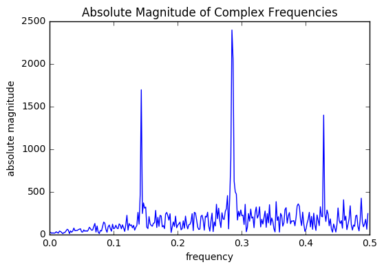
Taking the FFT of the time differenced signal creates a complex magnitude representation for each sinusoidal frequency component in the signal.
The data is filtered to include only the dominant sinusodial frequency components. Usually, the complex magnitude can be used to find the phase and absolute magnitude of the sinusodial wave corresponding to each frequency. In this case, we are using a time difference variable so the magnitudes and phases are not representative of the actual variable.
This process can be semi-automated by using statistics. The center frequency can be found by average across all frequencies. The bandwidth of the filter can be defined by frequencies within to standard deviations of the mean of the absolute complex magnitude. The purpose of this is avoid periods that are too large.
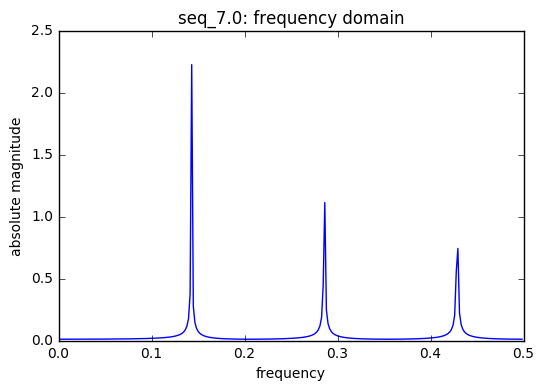
N = len(time_diff_signal)
unfiltered  = DSP.get_frequency_domain(time_diff_signal)
y_abs=( 2.0/N * np.abs(unfiltered[1:,1]))

center = np.mean(unfiltered[1:,0])
band = 1*np.std(unfiltered[1:,0])
threshold = np.mean(y_abs)+1*np.std(y_abs)

print("Center frequency: ",np.abs(center),"Band: ",np.absolute(band),"Threshold: ",threshold)

plt.plot(unfiltered[1:,0],y_abs)
plt.xlabel('frequency')
plt.ylabel('absolute magnitude')
plt.title("Absolute Magnitude of Complex Frequencies")
plt.show()

print("Frequency, Magnitude")
abs_filtered = np.absolute(DSP.filter_freq_domain(unfiltered, center,band,threshold))
print(abs_filtered)
Center frequency: 0.249568221071 Band: 0.14358883867 Threshold: 408.870795735
    Frequency, Magnitude
    [[  1.41623489e-01   1.33800535e+05]
     [  1.43350604e-01   4.90313504e+05]
     [  2.78065630e-01   1.31154698e+05]
     [  2.81519862e-01   1.23147724e+05]
     [  2.83246978e-01   2.54959357e+05]
     [  2.84974093e-01   6.93085781e+05]
     [  2.86701209e-01   5.95979105e+05]
     [  2.88428325e-01   1.80149377e+05]
     [  2.90155440e-01   1.44095857e+05]
     [  2.91882556e-01   1.36036705e+05]]
Creating seasonal predictor variables
After filtering the data, the dominant frequencies were found at .143, .28, and .29. These correspond to T=7,4, and 3, respectively. Sequences with these periods can be created.
Notice that the frequency .428, that corresponds to a period of 2 (actually a little below), was not included in our predictors. This is because of Nyquist's thoeorm:
"When the signal bandlimited to ? fs cycles/second (hertz), its Fourier transform, X(f), is 0 for all |f| > 1/2*(1/T)"
In this case the signal has a sampling period of 1 or a sampling frequency of 1. The maximum frequency we can "see," by Nyquist's theorm, would be a signal with a period greater than 2.
period_list = set([round(1/(ft)) for ft,ht in abs_filtered if round(1/(ft))>2])
print("Sequence list: ",period_list)

train = DSP.get_sequences(train,period_list,start_index=1,plot=True)
valid = DSP.get_sequences(valid,period_list,start_index=len(train)+1,plot=False)
valid.head()
Sequence list: {3.0, 4.0, 7.0}
| Day | Sessions | Pageviews | time | index | weekday | W_2 | W_3 | W_4 | W_5 | W_6 | W_7 | seq_3.0 | seq_4.0 | seq_7.0 | |
|---|---|---|---|---|---|---|---|---|---|---|---|---|---|---|---|
| 580 | 4/28/15 | 13162 | 19757 | 2015-04-28 | 581 | 2 | 1.0 | 0.0 | 0.0 | 0.0 | 0.0 | 0.0 | 2.0 | 1.0 | 0.0 |
| 581 | 4/29/15 | 12395 | 18568 | 2015-04-29 | 582 | 3 | 0.0 | 1.0 | 0.0 | 0.0 | 0.0 | 0.0 | 0.0 | 2.0 | 1.0 |
| 582 | 4/30/15 | 12351 | 19122 | 2015-04-30 | 583 | 4 | 0.0 | 0.0 | 1.0 | 0.0 | 0.0 | 0.0 | 1.0 | 3.0 | 2.0 |
| 583 | 5/1/15 | 12301 | 19830 | 2015-05-01 | 584 | 5 | 0.0 | 0.0 | 0.0 | 1.0 | 0.0 | 0.0 | 2.0 | 0.0 | 3.0 |
| 584 | 5/2/15 | 9345 | 14110 | 2015-05-02 | 585 | 6 | 0.0 | 0.0 | 0.0 | 0.0 | 1.0 | 0.0 | 0.0 | 1.0 | 4.0 |
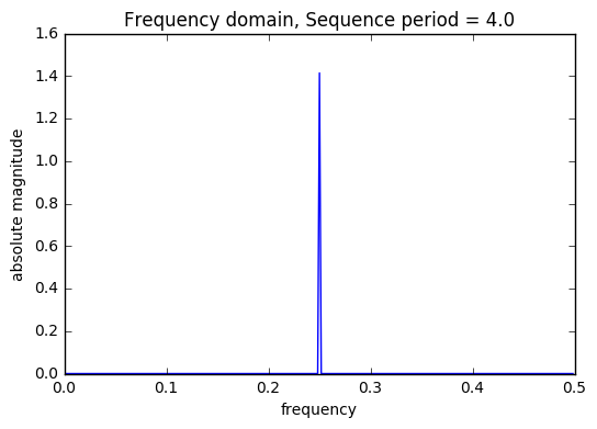
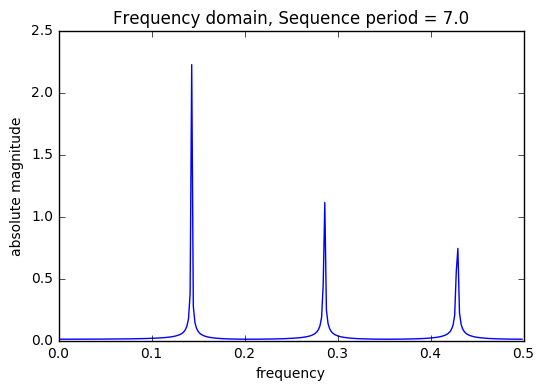
Eureka! Weekday (Sequence period = 7) shares the same frequency components as Pageviews!
The table below shows the index and weekday to help illustrate what the periods or cycles. The index starts at 1, but this corresponds to weekday 3 (or Wednesday). So index 6 corresponds to Monday and index 2 corresponds to Thursday.
Fitting the Model
Since T(t) is already created, this part of the blog will focus on S(t).
Each generated sequence will be made into pairs of seasonable components and will have at least two components, two sinusoidal waves, i.e. ?1sin(t/T) + ?2cos(t/T). In fact, the sum of weighted cosine & sine terms for each dominant frequency in the signal can be thought of as a Fourier Series. The difference is that the ? valus will only be estimated for the most dominant frequenciesinstead of an infinite, or large number of periodic waves.
Fourier series formula
How is this done automatically?
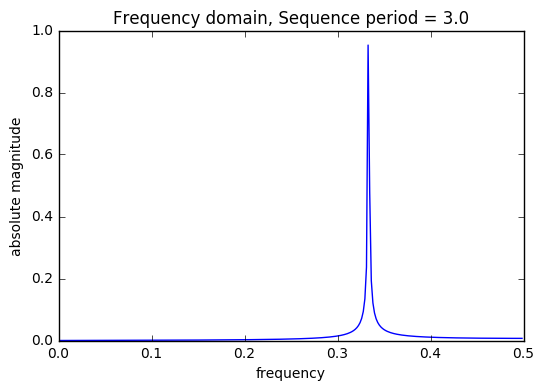
Consider an example where there exists a periodic signal of period 13 inside of the main signal.
Seasonal components are generated automatically by first creating a saw tooth wave with a period of 13. This series represent the time component of a series of sinusoids with various periods. But how do we choose these periods? The saw tooth wave is unique in that each level appears only once in each period. By taking the FFT of this wave, the frequencies of this wave show how many sinusoids are needed to represent the wave at each unique level. By selecting the dominany freuquencies of this wave, a variery of shapes can be create for the seasonal component of period 13. This is accomplished by summing a set of orthogonal sine waves, with different periods, which use the save tooth wave as the time component. The saw tooth wave is used at the time component to force the resultant wave to have a period of 13.
Sum of Cosines = β1sin(2*π*x/13) + β2cos(2*π*x/7) + β3cos(2*π*x/4) + β4cos(2*π*x/3) + β5cos(2*π*x/2) , 0 <= x < 13
output=train[['Pageviews']]
y=output.values

m,n =np.shape(output)
count=0


S_train = np.ones((len(train),1))
S_valid = np.ones((len(valid),1))

for component in period_list:
    f=DSP.get_sequence_freq(var=train[["seq_"+str(component)]],std_thresh=3,plot=True)
    x=DSP.get_seasonal_predictors(train[["seq_"+str(component)]],f)
    S_train=np.column_stack((S_train,x))
    x=DSP.get_seasonal_predictors(valid[["seq_"+str(component)]],f)
    S_valid=np.column_stack((S_valid,x))
    count+=1
plt.plot(train['index'][:60],train['Pageviews'][:60],'-')
plt.xlabel("time")
plt.ylabel("Pageviews")
plt.title("Pageviews")
plt.show()

x=S_train

A=x.T.dot(x)
b=x.T.dot(y)
z = np.linalg.solve(A,b)

SSE=np.sum((y-x.dot(z))**2)
print("SSE :",SSE)
print("Baseline: ",sum((y-np.mean(y))**2)[0])

# plt.plot(train['index'],y,'.')
plt.plot(train['index'][:60],x.dot(z)[:60],'-')
plt.title("Weighted Addition of Seasonal Components")
plt.xlabel("time")
plt.ylabel("predicted value")
plt.show()
print("coefficients: ")
print(z)
    threshold 0.213708597747
    frequencies  [[  0.00000000e+00   5.80000000e+02]
     [  3.31034483e-01   6.86580342e+01]
     [  3.32758621e-01   2.76353001e+02]
     [  3.34482759e-01   1.39043662e+02]]
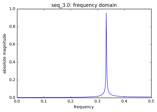
    frequencies used in  seq_3.0  :  [0.33333333333333331]
    frequencies used in  seq_3.0  :  [0.33333333333333331]
    threshold 0.254028420631
    frequencies  [[  0.00000000e+00   8.70000000e+02]
     [  2.50000000e-01   4.10121933e+02]]
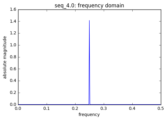
    frequencies used in  seq_4.0  :  [0.25]
    frequencies used in  seq_4.0  :  [0.25]
    threshold 0.525113865983
    frequencies  [[  0.00000000e+00   1.74300000e+03]
     [  1.43103448e-01   6.45133516e+02]
     [  2.86206897e-01   3.22688369e+02]
     [  4.27586207e-01   1.61660579e+02]
     [  4.29310345e-01   2.15278734e+02]]
    frequencies used in  seq_7.0  :  [0.14285714285714285, 0.5, 0.33333333333333331]
    frequencies used in  seq_7.0  :  [0.14285714285714285, 0.5, 0.33333333333333331]
    SSE : 5765825922.99
    Baseline:  8530795814.65
        coefficients:
    [[  1.06306549e+04]
     [ -1.63450638e+00]
     [  5.94252422e+01]
     [ -6.20595993e+01]
     [ -3.09144366e+00]
     [  1.29084218e+03]
     [ -5.98934835e+18]
     [ -2.34003768e+03]
     [  1.42249877e+03]
     [ -1.72123723e+03]
     [  1.13494916e+03]]
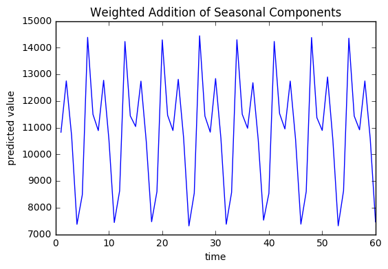
Weighted Addition of Seasonal Components
In the regression model, each of these components will get a weight associated with it which can be added together to create a weighted seasonal component. The weighted seasonal component has a pattern similar to that of the Pageviews.
Seasonal Predictors
There are 3 saw tooth sequences included in the model each with a unique t, time index. A saw tooth of period 3 & 4 have only two sinusoids with with periods 0.33 & 0.25, respectively. Finally, a saw tooth wave of period 7 is used inside of 6 sinusoids with periods 0.1428, 0.333, and 0.5.
These periods can be found using the same semi-automated techniques used to generate the sequences as described earlier. The threshold can be adjust by the number of standard deviations from the mean of the absolute complex magnitude.
Finding peaks
There are two peaks which correspond to Monday and Thursday. This is consistent with the problem solution given above.
peaks=[]
for i,xz in enumerate(x.dot(z)):
    if i>0 and i<len(x.dot(z))-1:
        if x.dot(z)[i]>x.dot(z)[i-1] and x.dot(z)[i]>x.dot(z)[i+1]:
            peaks.append(train['time'][i].isocalendar()[2])
print(set(peaks))
{1, 4}
Training & Validation
The following models will be trained and validated with different seasonal variables:
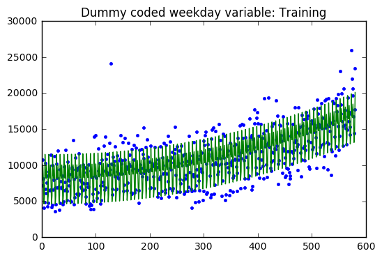
1. Model fitted with a dummy coded weekday variable
2. Model fitted with extracted sinusodial components
y=train[['Pageviews']].values

m =len(train)

x=np.ones((m,9))
x[:,1:]=np.column_stack((train['W_2'],train['W_3'],
                         train['W_4'],train['W_5'],train['W_6'],
                         train['W_7'],T_train))


A=x.T.dot(x)
b=x.T.dot(y)
z = np.linalg.solve(A,b)

SSE=np.sum((y-x.dot(z))**2)
SST=sum((y-np.mean(y))**2)[0]
print("Training")
print("SSE: ",SSE)
print("SST: ",SST)
print("R^2: ",1-SSE/SST)
print("Baseline: ",sum((y-np.mean(y))**2)[0])

plt.plot(train['index'],y,'.')
plt.plot(train['index'],x.dot(z),'-')
plt.title("Dummy coded weekday variable: Training")
plt.show()

plt.scatter(train['index'],y-x.dot(z))
plt.title("Residuals")
plt.show()
print("coefficients:")
print(z)
print()

y=valid[['Pageviews']].values

m =len(valid)

x=np.ones((m,9))
x[:,1:]=np.column_stack((valid['W_2'],valid['W_3'],
                         valid['W_4'],valid['W_5'],valid['W_6'],
                         valid['W_7'],T_valid))


SSE=np.sum((y-x.dot(z))**2)
SST=sum((y-np.mean(y))**2)[0]
print("Validation")
print("SSE: ",SSE)
print("SST: ",SST)
print("R^2: ",1-SSE/SST)
print("Baseline: ",sum((y-np.mean(y))**2)[0])

plt.plot(valid['index'],valid[['Pageviews']],'.')
plt.plot(valid['index'],x.dot(z),'-')
plt.title("Dummy coded weekday variable: Validation")
plt.show()

plt.scatter(valid['index'],y-x.dot(z))
plt.title("Residuals")
plt.show()
    Training
    SSE:  1912154025.09
    SST:  8530795814.65
    R^2:  0.775852796546
    Baseline:  8530795814.65
    coefficients:
    [[  1.15385953e+04]
     [ -2.79933336e+03]
     [ -3.32862564e+03]
     [ -1.48611482e+03]
     [ -3.71268360e+03]
     [ -6.88505486e+03]
     [ -5.73875872e+03]
     [ -1.29164524e+00]
     [  2.77465319e-02]]

    Validation
    SSE:  1159104596.32
    SST:  2424981317.62
    R^2:  0.522015040734
    Baseline:  2424981317.62
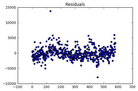
The regression model on the training dataset had an R-Squared value of 0.78 with 9 predictor variables. The residual are evenly distributed around zero with a two large outliers.
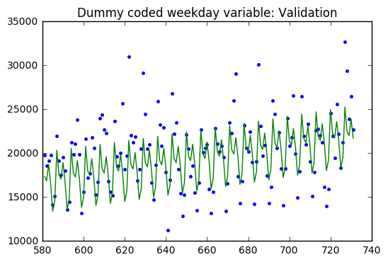
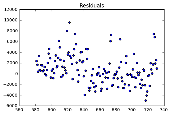
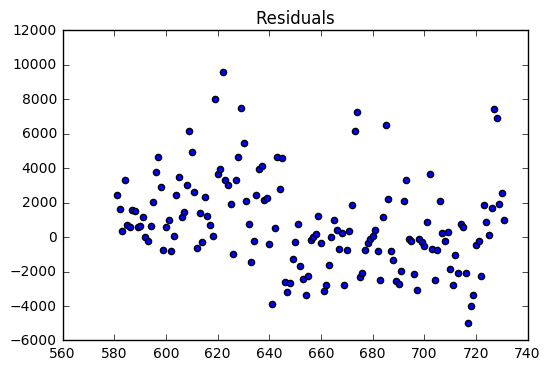
The validation dataset had an R-Squared of 0.52. The validation dataset residuals have many outliers compared the the training dataset residuals. In addition, there is a slight downward trend which suggests that a variable might be left out of the model.
y=train[['Pageviews']].values

x=np.column_stack((S_train,T_train))


A=x.T.dot(x)
b=x.T.dot(y)
z = np.linalg.solve(A,b)

SSE=np.sum((y-x.dot(z))**2)
print("SSE :",SSE)
print("Baseline: ",sum((y-np.mean(y))**2))


SSE=np.sum((y-x.dot(z))**2)
SST=sum((y-np.mean(y))**2)[0]
print("SSE: ",SSE)
print("SST: ",SST)
print("R^2: ",1-SSE/SST)


plt.plot(train['index'],y,'.')
plt.plot(train['index'],x.dot(z),'-')
plt.title("Seasonally predicted Values over time: Training")
plt.show()

plt.scatter(train['index'],y-x.dot(z))
plt.title("Residuals")
plt.show()


print(z)
print()


output=valid[['Pageviews']]
y=output.values


x=np.column_stack((S_valid,T_valid))

SSE=np.sum((y-x.dot(z))**2)
SST=sum((y-np.mean(y))**2)[0]

print("SSE: ",SSE)
print("SST: ",SST)
print("R^2: ",1-SSE/SST)
print("Baseline: ",sum((y-np.mean(y))**2)[0])

plt.plot(valid['index'],y,'.')
plt.plot(valid['index'],x.dot(z),'-')
plt.title("Seasonally predicted Values over time")
plt.show()
plt.scatter(valid['index'],y-x.dot(z))
plt.title("Residuals")
plt.show()

    SSE : 1910499966.56
    Baseline:  [  8.53079581e+09]
    SSE:  1910499966.56
    SST:  8530795814.65
    R^2:  0.776046689187
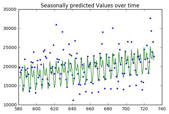
    SSE:  1160469260.63
    SST:  2424981317.62
    R^2:  0.521452288231
    Baseline:  2424981317.62
Results
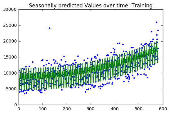
The regression model on the training dataset had an R-Squared value of 0.78 with 9 predictor variables. The residual are evenly distributed around zero with a two large outliers.
The validation dataset had an R-Squared of 0.52. The validation dataset residuals have many outliers compared the the training dataset residuals. In addition, there is a slight downward trend which suggests that a variable might be left out of the model.
The results are almost (if not) exactly the same, so which method to choose?
Dummy coding can be automated, but its not always easy to type every variable to include in a linear model. In addition, it requires some inpection and trail and error to find the seasonal variable. The advantage of dummy coding is that each level is accounted for and it relatively easy to compare levels.
Signal processing can be used to create seasonal components almost automatically, but it is more computational expensive to calculate. In addition, it is not clear from the coefficients what the seasonal components are. The advantage is that there can be more predictive variables in the model, and the number of sinusodial components can be increased or decreased by adjusting the threshold or bandwith.